The spectrogram is a standard sound visualization tool, showing the distribution of energy in both time and frequency. It is simply an image formed by the magnitude of the short-time Fourier transform, normally on a log-intensity axis (e.g. dB).
Matlab's Signal Processing Toolbox has a built-in specgram function, but to support students who had not purchased that toolbox, I wrote a drop-in replacement.
The return value of specgram is a complex array that contains enough information to fully reconstruct the original signal. I've written an inverse routine, ispecgram that will recreate sound from a (possibly modified) output of specgram.
For contrast, I've also written a function to plot spectrograms on a log-frequency axis. This isn't a very sophisticated version - it just performs a mapping of the linear-frequency bins from the FFT (rather than, say, varying the time window at different frequencies). But it shows the differences in this kind of display well enough.
I've included a second version of this log-frequency mapping, also known as constant-Q (i.e. the bandwidth-to-center-frequency ration is constant). This version attempts to preserve information enough information in the log-frequency domain to reconstruct the linear-frequency spectrogram with minimal distortion, to allow iterative mapping between the two spectral axes.
The code fragment below makes a simple comparison of linear and log-frequency spectrograms.
The routines provided here are:
An example use is shown below:
>> % Load a speech waveform
>> [d,sr] = wavread('sf2_cln.wav');
>>
>> % Conventional (linear-frequency) spectrogram
>> subplot(311)
>> specgram(d,1024,sr);
>> % Log-frequency spectrogram
>> subplot(312)
>> logfsgram(d,1024,sr);
>> % Recover approx to lin-F from log-F
>> [Y,MX]=logfsgram(d,1024,sr);
>> DR = sqrt(MX'*(Y.^2));
>> subplot(313)
>> imagesc(20*log10(DR))
>> caxis([-100 30])
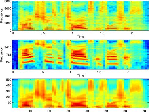
Notice how the bottom quarter of the lin-freq specgtrogram is expanded to almost all of the log-freq spectrogram, and how the sets of harmonic partials that are equally-spaced but stretching apart on the left become a pattern of unequally-spaced features moving in parallel on the right. Also notice how mapping the log-resolution spectrogram back to the lin-freq bins (with the MX mapping matrix returned by logfsgram) results in blurring in the higher frequency bins.
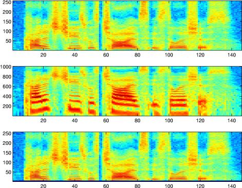
Here's an example of using the logfmap matrix:
>> % Start with the basic (linear-freq) spectrogram matxix
>> D = log(abs(specgram(d,512)));
>> % We're going to do the mapping in the log-magnitude domain
>> % so let's shift D so that a value of zero means something.
>> minD = min(min(D));
>> D = D - minD;
>> subplot(311)
>> imagesc(D); axis xy
>> c = caxis;
>>
>> % Design the mapping matrix to lose no bins at the top but 5 at the bottom
>> [M,N] = logfmap(257,6,257);
>> size(M)
ans =
        1006         257
>> % Our 257 bin FFT expands to 1006 log-F bins
>> % Perform the mapping:
>> MD = M*D;
>> subplot(312)
>> imagesc(MD); axis xy
>> caxis(c);
>> % Map back to the original axis space, just to check that we can
>> NMD = N*MD;
>> subplot(313)
>> imagesc(NMD); axis xy
>> caxis(c)
>> % Most bins look the same, except for the band that we lost at the bottom
This code is released under the BSD 2-clause license; see LICENSE.txt.